
by: Zank, CEO of Bennett Data Science
Last time, we looked at the importance of testing and showed how to save money and do it the right way. The method we showed is the Multi Armed Bandit (MAB). In this companion article, we’ll use a simple example to show you a handful of MAB options and how the Multi-Armed Bandit with Thompson Sampling outperforms them all.
Let’s Start with a simple Example:
Imagine you are running a marketing campaign for your website and have two ads to choose from. And say the objective is to show the ad with highest click through rate (CTR) to drive the highest traffic possible. But you don’t have any prior information about how either of these ads will perform. What would be your approach?
Sounds like a case for A/B testing, right? How about showing both of the ads equally to lots of users, then, at some point, switching to the ad with the highest measured CTR? How long do you have to show both ads before settling on a “winner”? In these cases, it seems like guessing might be our best bet. In fact, that’s not far off!
As we discussed last time, there’s a method for this very problem; it’s called the multi armed bandit (MAB).
There’s a lot of information explaining what the MAB algorithm is, what it does and how it works, so we’ll keep it brief. Essentially, the MAB algorithm is a near-optimal method for solving the explore exploit trade-off dilemma that occurs when we don’t know whether to explore possible options to find the one with the best payoff or exploit an option that we feel is the best, from the limited exploration done so far.
In this post, we’ll look at different algorithms that solve the MAB problem. They all have different approaches and different ways to approach Exploration vs Exploitation.
Let’s define a couple terms, that you may be familiar with:
- CTR – the ratio of how many times an ad was clicked vs. the number of impressions. For example, if an ad has been shown 100 times and clicked 10 times, CTR = 10/100 = 0.10
- Regret – the difference between the highest possible CTR and the CTR shown. For example, if ad A has a known CTR or 0.1 and ad B has a known CTR of 0.3, each time we show ad A, we have a regret equal to 0.3 – 0.1 = 0.2. This seems like a small difference until we consider that an ad may be shown 1MM times in only hours.
There are a few popular options for MAB’s. The four implementations we’ll use are:
- Random Selection
- Epsilon Greedy
- Thompson Sampling
- Upper Confidence Bound (UCB1)
We’re interested in finding the one that achieves the smallest regret. Each method will be described below in the simulations.
Some tech details:
To perform this experiment, we have to assume we know the CTR’s in advance. That way, we can simulate a click (or not) of a given ad. For example, if we show ad A, with a known CTR of 28%, we can assume the ad will be clicked on 28% of the time and bake that into our simulation.
ONE – Random Selection
- 0% – Exploration
- 100% – Exploitation
Let’s start with the most naïve approach – Random Selection. The Random Selection algorithm doesn’t do any Exploration, it just randomly chooses the Ad to show.
You can think of it as coin flip – if you get heads you show AdA, if you get tails you show Ad B. So if you have two ads, each will appear around 50% of the time. There are clear disadvantages of this model, but it’s an effective way to create a baseline from which to rate the other models.
Here are the simulation results, plotted. The top plot shows CTR values for options A & B. When the lines stop wiggling, it means the algorithm has strong confidence that it’s showing the right option. The lower plot shows the regret. Optimally we’d like this to be zero for each trial. That would mean we’re showing the correct option each time.
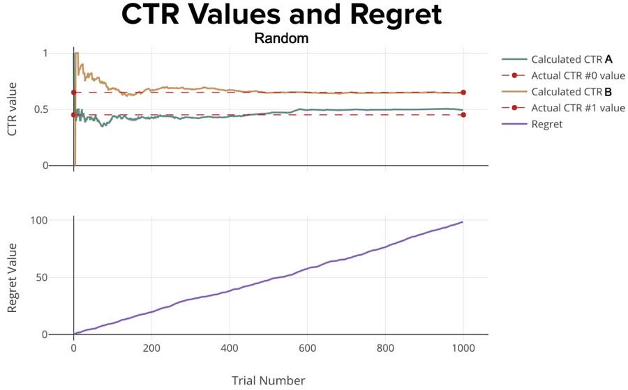
You can see the Regret increases continually since the algorithm doesn’t learn anything and doesn’t do any updates according to gained information. This ever-increasing regret is exactly what we’re hoping to minimize with “smarter” methods.
You might use this algorithm if you:
- Want to be confident about the estimated CTR value for each Ad (the more impression each Ad get, the more confident you are that estimated CTR equals to real CTR).
- Have unlimited Marketing Budget 😉
TWO – Epsilon Greedy
- ~15% – Exploration
- ~85% – Exploitation
The next approach is the Epsilon-Greedy algorithm. Its logic can be defined as follows:
- Run the experiment some initial number of iterations (Exploration).
- Then choose the winning variant with the highest score.
- Set the Epsilon value, ϵ.
- Run the experiment, choosing the winning variant for (1−ϵ)% of the time and other options for ϵ% of the time (Exploitation).
Translation? You always leave room for exploration. So, even if you have a “winner” the algorithm will continue to send some amount of traffic to the wrong option. That increases regret, as we’ll see:
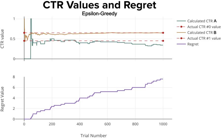
That’s much better; Notice how the regret has decreased by an order of magnitude! The Epsilon-Greedy algorithm seems to perform much better than Random Selection. But can you see the problem here? The winning variant will not necessarily be the optimal variant, and you actually still show the suboptimal variant. This increases regret and decreases reward.
According to the Law of Large Numbers* the more initial trials you do, the more likely you will choose the winning variant correctly. But in Marketing you don’t usually want to rely on chance and hope that you have reached that ‘large number of trials’.

*In probability theory, the Law of Large Numbers is a theorem that describes the result of performing the same experiment a large number of times. According to the law, the average of the results obtained from a large number of trials should be close
to the expected value, and will tend to become closer as more trials are performed.
It’s also why Las Vegas is so big and golden. In the end, the house always wins!
It’s possible to adjust the ratio that controls how often to show the winning ad after initial trials by choosing different ϵ values. But who wants to do that?!
THREE – Thompson Sampling
- 50% – Exploration
- 50% – Exploitation
Thompson Sampling exploration part is more sophisticated than e-Greedy algorithm. It’s rather complex to explain, but much more straightforward to implement, so we’ll leave out the details and get right to the results.
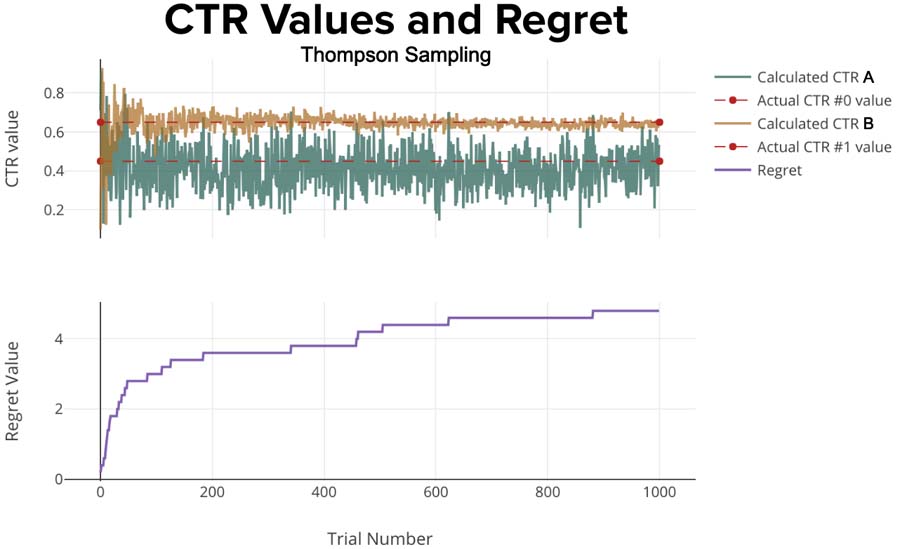
The regret is the lowest we’ve seen so far. Each uptick in regret happened when Ad A (the wrong Ad) was chosen. In the bottom plot, you see the regret comes up quickly in the first 75 trials and after that, Ad A is rarely shown (causing small amounts of additional regret).
FOUR – Upper Confidence Bound (UCB1)
- 50% – Exploration
- 50% – Exploitation
Unlike the Thompson Sampling algorithm, the Upper Confidence Bound cares more about the uncertainty (high variation) of each variant. The more uncertain we are about one variant, the more important it is to explore. Intuitively, that makes sense.
The logic is rather straightforward:
- Calculate the UCB for all variants.
- Choose the variant with the highest UCB.
- Go to 1.
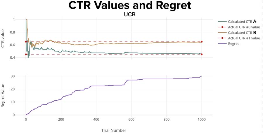
You can see that only the random model has worse regret.
Comparison and Conclusions
Now let’s compare four of this methods and see which one performed better for our problem.
It’s obvious that we want to show the Ad B more often since its actual CTR is 0.65. Let’s take a look at the ratio of how many time the right Ad has been chosen for each algorithm.
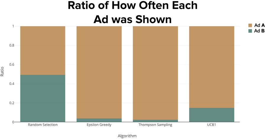 The winners here are Thompson Sampling and Epsilon-Greedy since they showed Ad B the highest percentage of the time.
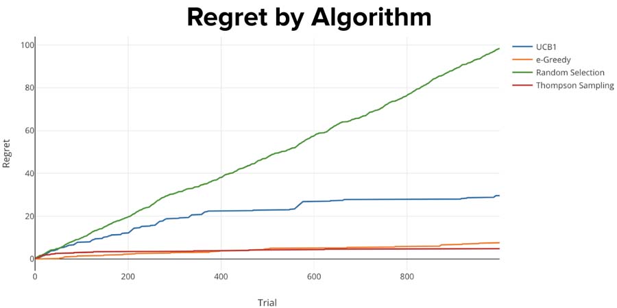
Taking into account that Thompson Sampling and Epsilon-Greedy algorithms chose ad with the higher CTR most of the time, it shouldn’t come as surprise that their regret values are the lowest.
Finally, we look at the opposite of regret, reward. It can happen that the algorithm with the lowest regret does not have the highest reward. This is because even if the algorithm chooses the right ad, there is no guarantee that the user will click on it.
Conclusion
Last time, we established the importance of testing the right way. Without mentioning it, we used the Multi Armed Bandit (MAB) with Thompson Sampling. Here’s we’ve shown, with a simple example, how a Multi-Armed Bandit with Thompson Sampling is generally the best choice for A/B tests in terms of minimizing regret.
At Bennett Data Science, we’re experts at A/B/n testing. We’d love to help you boost earnings by unlocking your potential by testing everything customer facing.
Zank Bennett is CEO of Bennett Data Science, a group that works with companies from early-stage startups to the Fortune 500. BDS specializes in working with large volumes of data to solve complex business problems, finding novel ways for companies to grow their products and revenue using data, and maximizing the effectiveness of existing data science personnel. https://bennettdatascience.com/staging