
We’re finally here: Part five of my series on Deploying Predictive Models. Here’s what I’ve covered so far:
- How deployment fits into a proven 10-step data science methodology
- Why deployment is an important part of any organization’s data science roadmap
- What a model is and how to consider deploying something simple
- The types of predictions and how they impact deployment concerns
This week, I’ll wrap the series up by looking at the metrics used to measure the accuracy of deployed models and how to make sure models don’t get stale because they will if not carefully attended to.
The performance of models is assessed by metrics. There are two scenarios where models are assessed, and each scenario is associated with specific metrics:
- Pre-deployment, during the modeling phase
- Post-deployment, when the model is in production
Both scenarios are vastly different. If you haven’t thought about this distinction before, you’re not alone. Many data scientists don’t even think about the difference. Let’s dive in.
Pre-Deployment
Pre-deployment performance is generally measured by assessing the ability of a predictive model to return accurate results on a hold-out set. Here’s what that usually looks like in the example of predicting home prices from square footage.
To understand the accuracy of our home price predictions in part three, a data scientist might collect 100,000 home prices and square footage values. From there, they would likely use 70,000 for training a model, then hold out the remaining 30,000 to validate the performance of the model.
In other words, the model is trained on the 70,000 values of home price and square footage. Then, using the remaining 30,000 values for square footage, the model predicts the price. Then, these predictions are compared with the actual prices. The difference between the predictions and the actual prices is the accuracy. And it can be measured in many ways using different metrics.
One metric to use is the “mean absolute error” (MAE). That’s the average distance between the predicted value and the actual value. It can be positive or negative. It’s quite easy to compute. This metric weighs all errors in the same way so that all individual differences have equal weight. In other words, an error of 10.0 would be ten times worse than an error of 1.0.
It’s very intuitive and using MAE can be appropriate, but what if you want to punish a model disproportionately more for making bigger errors? In that case, you might use something like the “root mean squared error” (RMSE) that does exactly that, by squaring the errors. RMSE gives a higher weight to larger errors. We generally use RMSE when large errors are particularly undesirable.
The point is not to define performance metrics here, but to show that the choice of offline performance metrics matters and early decisions need to be made so data scientists know how their models’ performance will be measured.
Post-Deployment
Post-deployment metrics are usually very different. These tend to be Key Performance Indicators (KPIs), such as increased engagement or reduced churn rate.
The million-dollar question is this: how in the world does a good value of “mean absolute error” in pre-deployment testing help me understand how my engagement will increase?
That’s a great question! The answer is, we don’t know. In the case of predicting home prices from square footage, we’re hoping that accurate results will result in more time spent on site and more shares across social media. But ultimately we don’t know.
In this case, we assume that a low “mean absolute error” is a proxy for increased engagement. If you don’t buy that assumption, I don’t blame you; it’s a big leap. But what else can we do? How else can data scientists optimize for engagement when we don’t have any data tying home price prediction to customer engagement?
In many cases, a proxy is all we have. And in many cases, it’s enough to help data scientists build a model that performs well enough. And well enough is, um, well enough!
But we can do better.
And that’s where continuous optimization comes in.
Continuous optimization
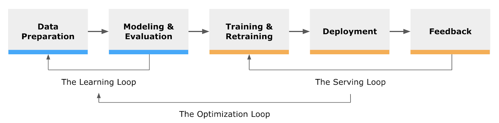
This above diagram shows two important stages: the Serving Loop and the Optimization Loop.
The Serving Loop is how most companies retrain their models each day (or hour/week/month) to keep things fresh. The Optimization Loop refers to the process of going all the way back to the modeling phase to create new models that will hopefully increase performance. It’s this optimization stage that can deliver real-world gains.
Where offline testing might show increases in a proxy of real KPI’s, only by building and deploying new models can we show measurable increases in KPI’s.
It’s worth mentioning that without implementing the Optimization Loop, model accuracy can (and almost always will) drift and performance will degrade. This rarely happens with the presence of the Optimization Loop, but without this step, events like changes in seasons or drastic stock reductions can lower accuracy and cause a drop in user/customer engagement.
For these reasons, I always recommend making sure that data scientists stay involved with the upkeep of deployed models.
Checklist
Finally, here’s my checklist for successfully protecting your investment in data science by making sure your models make it to deployment and beyond:
- Have early conversations to establish objectives and a deployment contract
- Decide whether to use online or batch predictions
- Establish a go/no-go for model accuracy before deployment
- Establish metrics to be used to monitor deployed models and ways to measure them
- Establish a plan to develop alternate models for continuous improvement through variant testing
Much of what I talked about was high-level and covered good principles for deploying data science models. I encourage you to use this information to guide early conversations with your team, thus minimizing surprises and delays in realizing big value from predictive analytics.
That’s it for the Deploying Predictive Models series folks! I hope that this was helpful. Please let me know what you think, and if you have any remaining questions, I’m happy to answer those. Be well!
Best,
Zank
Of Interest
How Data Analysis, A.I. and IoT will Shape the Post-Pandemic ‘New Normal’
When a contagion is raging, grassroots responses can be counterproductive if everybody’s operating at cross-purposes. Lack of central coordination can confuse the situation for everybody, stoking a panic-driven infodemic that social media can exacerbate, drowning out guidance from public health officials and other reliable sources. To ensure effective orchestration of community-wide responses to a contagion, there is no substitute for authoritative data analytics to drive effective responses at all levels of society.
https://www.infoworld.com/article/3543770/how-data-analysis-ai-and-iot-will-shape-the-post-pandemic-new-normal.html
The Dumb Reason Your A.I. Project Will Fail
When companies pour huge amounts of time and resources into thinking about their A.I. models, they often do so while failing to consider how to make the A.I. actually work with the systems they have. This is an unnecessary mistake that can be prevented with the right approach. Read more here:
https://hbr.org/2020/06/the-dumb-reason-your-ai-project-will-fail
The Global A.I. Agenda: Latin America
While Latin American businesses are adopting A.I. at scale, the lack of regional cohesion and political stability are ultimately holding the ecosystem back. Read more about the Global A.I. Agenda’s findings on Technology Review:
https://www.technologyreview.com/2020/06/08/1002864/the-global-ai-agenda-latin-america/